Labelled transition systems
An LTS consists of a set of states and a set of transitions between those states. These transitions are labelled by actions and one state is designated as the initial state.
Formally, an LTS is a tuple \((S, A, \to, s_0)\) where:
\(S\) is a (finite) set of states;
\(A\) is a set of actions;
\(\to \subseteq S \times A \times S\) is a transition relation;
\(s_0 \in S\) is the initial state.
For any set of actions \(A\) we denote by \(A^*\) the set of all finite sequences of elements of \(A\). An element of \(A^*\) is called an action sequence or trace and the empty trace is denoted by \(\epsilon\).
For any LTS \((S, A, \to, s_0)\), states \(s,t \in S\) and action sequence \(\sigma \in A^*\), with \(\sigma = a_1 \ldots a_n\) for some \(n \ge 0\), we denote by \(s \to^\sigma t\) the fact that there exist \(s_0 \ldots s_n \in S\) such that \(s = s_0\), \(t = s_n\), and \((s_i, a_{i+1}, s_{i+1}) \in \to\) for all \(0 \le i < n\). Note that for all states \(s\) it holds that \(s \to^\epsilon s\).
An LTS usually describes the (discrete) behaviour of some system or protocol: in any state of the system, a number of actions can be performed, each of which leads to a new state. The initial state corresponds to the state in which the system resides before any action has been performed.
This LTS model can be extended in various ways. We briefly describe the addition of internal actions and of state values below.
Internal actions
When studying the behaviour of a system, one often wants to view the system as a black box. Only the interactions of the system with its environment are of interest and all internal behaviour should be hidden. For this, a special action called the internal action is introduced. It is often designated by \(\tau\). The internal behaviour of a system can now be hidden by renaming all actions that it performs internally, to \(\tau\). In the LTS model, the \(\tau\) is a special label that can be carried by a transition.
We can then consider traces between states on which any number of \(\tau\) actions may occur in between; we do not care how many. For convenience we introduce additional notation to express this. Let \(\tau^*\) denote any finite sequence of \(\tau\) actions.
For any LTS \((S, A, \to, s_0)\), states \(s,t \in S\) and action sequence \(\sigma \in (A \setminus \tau)^*\), with \(\sigma = a_1 \ldots a_n\) for \(n \ge 0\), we denote by \(s \to^\sigma t\) the fact that there exist \(s_0 \ldots s_n \in S\) such that \(s = s_0, t = s_n\), and \(s_i \to^{(\tau^* a_{i+1})} s_{i+1}\) for all \(0 \le i < n\).
State values
The state of a system can be defined as the combination of the values of all relevant parameters or variables. Hence, the LTS model can be extended by associating a state vector with every state. This is the list of parameters along with their values in that specific state.
Formally, we write a state vector declaration as a tuple \((d_1: D_1, \ldots, d_n: D_n)\) where \(d_i\) is the name and \(D_i\) is the domain (the set of possible values) of parameter \(i\). The set of states of an LTS now becomes a subset of \(D_1 \times \ldots \times D_n\). Hence, every state is an n-tuple that contains one specific value for every declared parameter.
Equivalences
Given two LTSs, a natural question is whether they describe the same behaviour. To answer this question we must first specify what we mean by “the same”. For example, are we satisfied if both LTSs can perform the same sequences of actions (starting from their initial states) or do we want to impose stricter criteria? In other words, we have to specify when we consider two LTSs to be equivalent.
Various notions of equivalence have been defined in the literature. Some are finer than others, meaning that the criteria that two LTSs should meet for them to be called equivalent, are stronger. The equivalences that we consider here are explained in the following sections.
Trace equivalence
According to trace equivalence, two LTSs are equivalent if and only if they can perform the same sequences of actions, starting from their initial states.
Formally, for any LTS \((S, A, \to, s_0)\) and state \(s \in S\) we define \(\Tr{s}\) to be the set of traces possible from \(s\):
Given two LTSs \(T = (S, A, \to, s_0)\) and \(T' = (S', A', \to', s'_0)\), we say that \(T\) and \(T'\) are trace equivalent iff \(\Tr{s_0} = \Tr{s'_0}\).
Weak trace equivalence
Weak trace equivalence* is very similar to trace equivalence. The only difference is that it “skips” any \(\tau\) actions that appear on the traces. Hence, weak trace equivalence is particularly useful when some parts of the behaviour have been hidden.
For example, if one LTS describes the desired, external behaviour of a system and another LTS describes its implementation with internal actions renamed to \(\tau\), then a natural question would be whether the two LTSs are weakly trace equivalent. In this case, “normal” trace equivalence would be too strong.
Formally, for any LTS \((S, A, \to, s_0)\) and state \(s \in S\) we define \(\Trw{s}\) to be the set of weak traces possible from \(s\):
Given two LTSs \(T = (S, A, \to, s_0)\) and \(T' = (S', A', \to', s'_0)\), we say that \(T\) and \(T'\) are weakly trace equivalent iff \(\Trw{s_0} = \Trw{s'_0}\).
Obviously, if \(s \trans{\sigma} t\) then there exists a sequence \(\pi\) (possibly containing \(\tau\) steps) such that \(s \trans{\pi} t\). Using this fact, it is not hard to see that if two LTSs are trace equivalent then they are also weakly trace equivalent.
Strong bisimilarity
Strong bisimilarity (or strong bisimulation equivalence) relates two LTSs in the following way: if one LTS can perform an action \(a\) then the other LTS must also be able to perform an \(a\) action and in such a way that the resulting states are again related. This relation works both ways simultaneously (which is suggested by the “bi-” prefix in the name of the equivalence).
The formal definition is as follows.
A relation \(R\) on the states of an LTS is called a simulation if for any states \(s, s', t\) and action \(a\), if \(s \trans{a} s'\) and \(s \mathrel{R} t\) then there exists a state \(t'\) such that \(t \trans{a} t'\) and \(s' \mathrel{R} t'\).
A symmetric simulation is called a bisimulation.
Two states \(s\) and \(t\) are called strongly bisimilar (or strongly bisimulation equivalent) iff there exists a bisimulation \(R\) such that \(s \mathrel{R} t\).
Given two LTSs \(T = (S, A, \to, s_0)\) and \(T' = (S', A', \to', s'_0)\), we say that \(T\) and \(T'\) are strongly bisimilar iff \(s_0\) and \(s'_0\) are strongly bisimilar.
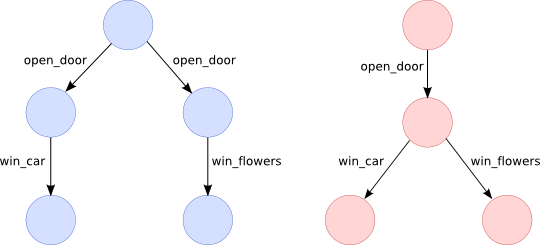
These LTSs are trace equivalent, but not strongly bisimilar.
Strong bisimilarity is a finer equivalence than trace equivalence, meaning it is stricter and relates less LTSs.
An example showing the difference between strong bisimilarity and trace equivalence is given in the figure above. These LTSs model a game show in which the contestant can open one of two doors to determine the prize he/she will win. Behind one is a very luxurious car, behind the other a nice bouquet of flowers. In the red model, the contestant can somehow still choose the prize after opening a door. In the blue model, the choice is made as soon as he/she opens a door.
According to trace equivalence, these models are equivalent. However, strong bisimilarity distinguishes the two: the blue model can simulate the open_door action by the red model, but in each of the resulting states it cannot simulate one of the win actions that the red model can perform.
Branching bisimilarity
Branching bisimilarity (or branching bisimulation equivalence) is a variant of strong bisimilarity that treats \(\tau\) actions in a special way. In cases where one of the LTSs under comparison contains internal actions, strong bisimilarity is often too strict and branching bisimilarity makes more sense.
The idea behind branching bisimilarity is that an LTS may skip \(\tau\) actions when simulating an action of the other LTS, but the intermediate states need to be related. (If the latter requirement is lifted, we obtain an equivalence known as weak bisimilarity.)
Branching bisimilarity is formally defined as follows.
A relation \(R\) on the states of an LTS is called a branching simulation if for any states \(s, s', t\) and action \(a\), if \(s \trans{a} s'\) and \(s \mathrel{R} t\) then:
either \(a = \tau\) and \(s' \mathrel{R} t\)
or there exist states \(t_1, t_2, t'\) such that \(t \trans{\tau^*} t_1 \trans{a} t_2 \trans{\tau^*} t'\) and \(s \mathrel{R} t_1, s' \mathrel{R} t_2\) and \(s' \mathrel{R} t'\).
A symmetric branching simulation is called a branching bisimulation.
Two states \(s\) and \(t\) are called branching bisimilar (or branching bisimulation equivalent) iff there exists a branching bisimulation \(R\) such that \(s \mathrel{R} t\).
Given two LTSs \(T = (S, A, \to, s_0)\) and \(T' = (S', A', \to', s'_0)\), we say that \(T\) and \(T'\) are branching bisimilar iff \(s_0\) and \(s'_0\) are branching bisimilar.
Isomorphism
One of the strongest equivalences is isomorphism. Two labelled transition systems are isomorphic if their structure is exactly the same. To compare, trace equivalence preserves a minimal amount of structure; only the order in which actions can occur is preserved. Bisimilarity, on the other hand, also preserves the branching structure.
Formally, two LTSs \(T = (S, A, \to, s_0)\) and \(T' = (S', A', \to', s'_0)\) are isomorphic if, and only if, \(A = A'\) and there is a bijective function \(f\) mapping states from \(S\) to \(S'\) such that \(f(s_0) = s'_0\) and \(s \trans{} s'\), for some \(s, s' \in S\), if and only if \(f(s) \trans{}' f(s')\).
Effectively this means that the isomorphic LTSs are only allowed to differ in their labelling of states.
Determinism
An LTS is called deterministic if for every state \(s\) and action \(a\), there is at most one state \(t\) such that \(s \trans{a} t\). (Note that in the classical definition of determinism, in the context of finite state acceptors, there should be precisely one such \(t\) for every \(s\) and \(a\).)
For example, in the figure above, the red LTS is deterministic, while the blue one is not.
For deterministic LTSs, trace equivalence and strong bisimilarity coincide. This means that two LTSs are trace equivalent if and only if they are strongly bisimilar. As mentioned before, for nondeterministic LTSs we do not have the only if part, just the if part.
We can also refer to determinism modulo an equivalence. We say an LTS \(l\) is deterministic modulo an equivalence \(e\) if, and only if, there is a deterministic LTS that is \(e\)-equivalent to \(l\). Note that modulo trace equivalence every LTS is deterministic and that the normal notion of determinism (i.e. without modulo) corresponds to determinism modulo isomorphism.